Perceptron: Basic Principles of Deep Neural Networks
Article information

Abstract
Big data, artificial intelligence, machine learning, and deep learning have received considerable attention in the medical field. Attempts to use such machine learning in areas where medical decisions are difficult or necessary are continuously being made. To date, there have been many attempts to solve problems associated with the use of machine learning by using deep learning; hence, physicians should also have basic knowledge in this regard. Deep neural networks are one of the most actively studied methods in the field of machine learning. The perceptron is one of these artificial neural network models, and it can be considered as the starting point of artificial neural network models. Perceptrons receive various inputs and produce one output. In a perceptron, various weights (ω) are given to various inputs, and as ω becomes larger, it becomes an important factor. In other words, a perceptron is an algorithm with both input and output. When an input is provided, the output is produced according to a set rule. In this paper, the decision rules of the perceptron and its basic principles are examined. The intent is to provide a wide range of physicians with an understanding of the latest machine-learning methodologies based on deep neural networks.
INTRODUCTION
Machine learning improves information processing ability through learning acquired through various processing experiences of data inputs into a computer program. Previously,1) machine learning was interpreted, in an informal manner, as “a field in which a machine attempts to derive a solution with high performance, for a specific problem, by applying a learning strategy to given data.” Along with extensive research on various types of machine learning, information technology (IT) related to data production, storage, and management has been developed.2)3) With the development of IT, machine learning in various fields, such as drug discovery,4) medical diagnosis,5) protein structure,6) and functionality7) prediction methodologies are being used successfully.
Machine learning can be largely grouped into supervised learning, unsupervised learning or reinforcement learning.8)9) Supervised learning is used to provide the correct answer in advance, with data already secured, and to learn it.10) Good examples to illustrate this are “if your blood pressure is high, then you have hypertension” or “if you have high blood pressure and diabetes, then the incidence of cardiovascular disease increases.” Similarly, supervised learning favors this “if–then” structure. In such supervised learning, there are “classifications” that classify and divide data according to a set rule, and “regression,” which predicts the result by finding a pattern.11)
In this article, the classification problem is discussed from the perspective of supervised learning, which is the most basic among machine-learning techniques and is most familiar to physicians. Decision trees are the most representative operating method, and the process is repeated continuously until a final diagnosis is made. Deep neural networks are one of the most actively researched and utilized methodologies in supervised learning. Machine learning is approached herein through a detailed explanation of the working principle of a “perceptron,” which is the basis of deep neural networks. In addition, this article is intended to help physicians in various fields to intuitively understand machine learning.
PRELIMINARY KNOWLEDGE ON TRAINING DATA EXPRESSED BY VECTORS
To gain insight into machine learning, it is necessary to understand the vectors representing data and basic operations on these vectors. Supervised learning refers to the process of deriving a function that provides an appropriate output when specific data are input. The data used in this process are called “training data,” and a typical form of the training data is shown in Table 1. Table 1 shows the data of 8 patients and consists of the results of 2 tests (tests A and B), that each patient received, together with the resulting diagnosis (+1: cardiovascular disease, −1: normal). At this time, each test is referred to as a “feature,” and the diagnosis result is referred to as a “label.” In summary, given the feature list (result values of tests A and B), a function to predict the appropriate label (whether the patient has cardiovascular disease or is normal) is derived based on the training data expressed in Table 1. This process is called “supervised learning.” “Learning” is the process of finding the pattern between the features and the label existing in the training data as a function.
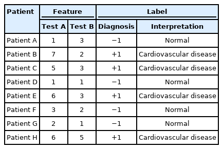
Typical form of the training data in supervised learning: diagnosis results, where “cardiovascular disease” and “normal” are denoted by +1 and −1, respectively
The training data in Table 1 can be expressed in a 2-dimensional space, as shown in Figure 1. The data C (5,3), in Figure 1, expressed on the coordinate system can be interpreted as a movement of 5 along the test A axis and 3 along the test B axis, with respect to the origin. Therefore, Table 1 can be described as a vector in a 2-dimensional space as follows (Figure 1): [{A[1,3], −1}, {B[7,2], +1},{C[5,3], +1}, {D[1,1], −1}, {E[6,3], +1}, {F[3,2], −1}, {G[2,1], −1}, {H[6,5], +1}].
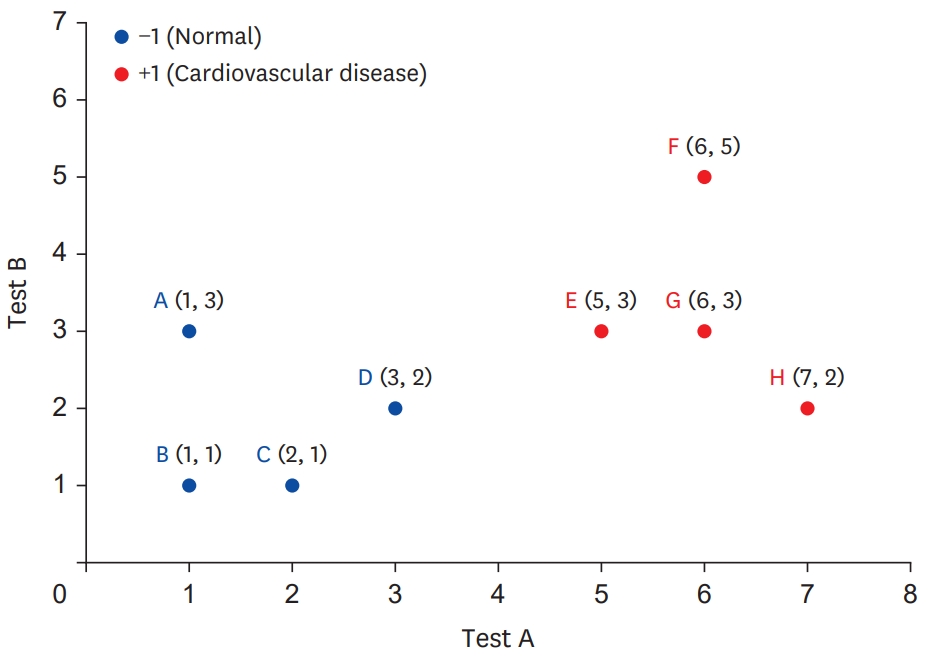
Training data expressed by vector in 2-dimensional space.
In general, a vector (Ʋ) described in the form of Ʋ=[Ʋ1, Ʋ2, Ʋ3, …, Ʋn] is a quantity having a direction and a magnitude. Each Ʋn is a component of Ʋ, where Ʋ is called an n-dimensional vector. Moreover, if each element of the vector Ʋ is multiplied by α, which is a positive number, a vector that is doubled by α, while maintaining the direction of the vector, is obtained. However, if α is a negative number, it is possible to obtain a vector that has a magnitude of α times the direction opposite to the existing direction. The notation |v| is used to indicate the magnitude of the vector and is calculated using Equation 1. One of the advantages of examining the training data from a vector point of view is that various operators related to vectors can be employed.
BASIC OPERATORS REQUIRED TO UNDERSTAND PERCEPTRONS
In this section, the addition, subtraction, and dot product of the vectors are briefly discussed. Addition, subtraction, and dot product for given 2-dimensional vectors Ʋ and Ư are defined as shown in Table 2. As can be seen in Table 2, the result of addition and subtraction between 2 n-dimensional vectors is another n-dimensional vector, whereas the result of the dot product is a single scalar value. In addition and subtraction, where the result of the operation is a new vector, as shown in Figure 2, the meaning of the operation can be understood and interpreted as a physical movement. Considering the addition of 2 vectors “Ʋ+Ư” as an example, it is interpreted as the direction and magnitude of moving along vector Ʋ from the origin and then additionally moving along Ư (the starting point of the vector is not necessarily the origin; however, it is assumed so for convenience).

Definitions of “addition,” “subtraction,” and “dot product” of vectors
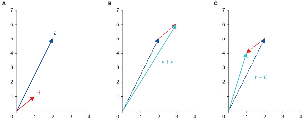
Understanding of the meaning of the operation as a physical movement. (A) Two dimensional sample vector
However, because the dot product of a vector is the result of a single number (scalar) operation, there is a limit to understanding its meaning through movement. Equation 2 defines the dot product of a vector as follows:
where θ is the difference in direction between Ʋ and Ư.
Equation 2 can be interpreted as reflecting the difference θ in the directions between vectors after multiplying the magnitudes of the vectors. Because the cosine graph has a value of 1 when θ is 0° (cos 0°=1), if the directions of the 2 vectors are the same, the dot product has the same result as multiplying the magnitudes of the 2 vectors. However, because the directions of the 2 vectors are different, the value of the vector dot product decreases. Furthermore, if it is an obtuse angle, a negative sign is used. As the magnitude of the vector cannot be negative, it can be recognized that the sign of the resulting value of the dot product operation, on the 2 vectors, is ultimately determined by the angle θ that formed between the 2 vectors.
PERCEPTRON AND THE DECISION RULE
The perceptron is a machine-learning methodology that can be regarded as the progenitor of deep neural networks.12)13) The perceptron utilizes 1-dimensional data (i.e., points), 2-dimensional data (lines), 3-dimensional data (planes), and 4-dimensional data (hyperplanes). The perceptron is a representative linear classifier model that bisects the space in which the training data exist in this manner.14)
As shown in Figure 3, the perceptron is a model that classifies the learning data existing in a 2-dimensional space using a straight line. One straight line, in the 2-dimensional space, is in the form of y=αχ+β using the slope α and the intercept β, and the point (χ0, y0) through which the straight line passes and the slope α based “y−y0=α(χ−χ0)” can be expressed in various ways. In this section, the most common (standard) form, αχ+βy=ƈ, is used for ease of explanation. At this time, because the constants α and β are weights, multiplied by the values of χ and y, α is substituted with ω1 and β with ω2. Furthermore, because the variables χ and y are arbitrarily assigned simple variable names, if χ1 and χ2 are replaced, the straight line in Figure 3 can be expressed as ω1χ1+ω2χ2=ƈ.
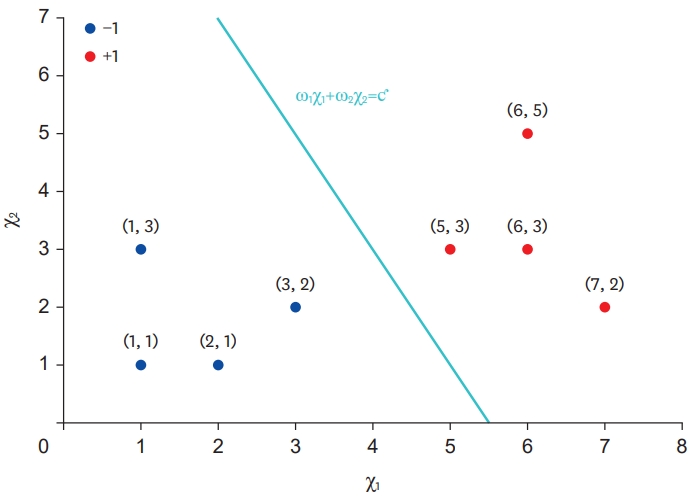
Model that classifies learning data in a 2-dimensional space using straight lines.
Among the training data shown in Figure 3, the 4 blue dots belonging to the normal class are the points where the result of the operation is smaller than ƈ when substituted into ω1χ1+ω2χ2. In addition, the 4 red dots can be interpreted as the points where the operation result is larger than ƈ. In other words, the perceptron shown in Figure 3 can be regarded as a model that divides a given space into −1 and +1 based on the straight line ω1χ1+ω2χ2=ƈ. This is described in more detail as follows.
The decision rule of the perceptron expressed in Equation 3 is limited to 2-dimensional data, that is, when data are described with 2 characteristics, χ1 and χ2. Therefore, if the classification rule of the perceptron is generalized and expressed in a form applicable to data existing in the n-dimensional space, it is expressed as Equation 4.
In addition, if χn+1 of a hypothetical (bias) having all values of “+1” and a corresponding weight ωn+1 (however, ωn+1=−ƈ) are given, Equation 4 is transformed, as shown in Equation 5.
Considering the decision rule of the perceptron expressed in Equation 6, it can be interpreted that the given data are classified according to the sign of
PERCEPTRON LEARNING ALGORITHM (PLA)
Previously, the classification rules used by the perceptron, to classify the given data, have been discussed. In this section, the derivation of a perceptron that perfectly classifies the given training data (red and blue dots), similar to the straight line in Figure 3, is discussed. In other words, the PLA is a method of finding a perceptron ω that perfectly divides “−1” and “+1” among countless candidates of perceptrons in space.
By inputting the training data D={(χ1, y1), (χ2, y2), (χ3, y4), …, (χƙ, yƙ)} composed of ƙ data, the PLA learns and returns the perceptron ω through the following process (Table 3). Similar to other machine-learning methodologies, the PLA randomly generates perceptron ω and then updates it to learn (line 1). Each datum belonging to the training data (line 5) is classified according to the perceptron decision rule described in Equation 6, and whether it matches the actual value (line 6) is checked. If even one data point is misclassified, the perceptron ω is updated (line 8). If all data are correctly classified, the training process ends, the update is completed, and ω is returned (line 13). In the end, the process of updating the current perceptron ω to “ω+y×χ” using the misclassified data (χ, y) is the core of learning. Understanding the effectiveness of this operation is essential. The update process is performed when “sign (ω·χ)≠sign (y)”, the condition described in line 6, is satisfied.

Perceptron learning algorithm
Figure 4A shows the case where the sign of the dot product operation (resulting from the data χ and the current perceptron ω, where the correct answer is −1 (y=−1) is positive. As mentioned, the sign of the resulting value of the inter-vector dot product operation is determined by the angle θ between the 2 vectors. As shown in Figure 4A, if the sign is positive, it is an acute angle. In other words, the current perceptron misclassifies the data ω because the angle θ, formed by the 2 vectors, is an acute angle. In this case, if ω is updated according to the perceptron update rule in line 8 (Table 3), the angle formed by the updated ω and χ becomes an obtuse angle, as shown in Figure 4A, and χ is correctly classified.
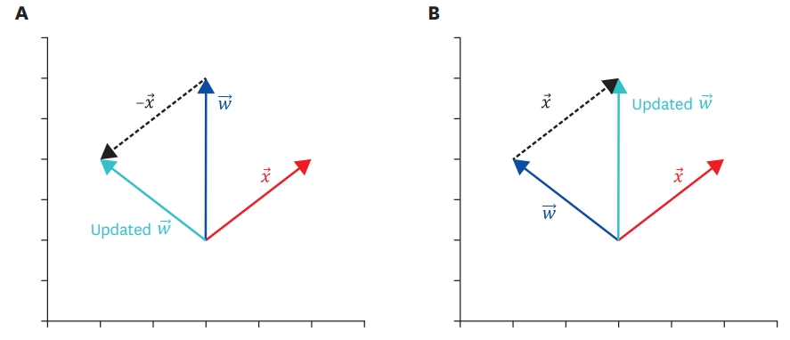
Perceptron update effect where blue
Figure 4B can be interpreted in a similar way. Figure 4B can be considered an error because θ, which is the difference in direction between the current perceptron ω, and the data where the correct answer is +1 (y=+1), is an obtuse angle. If θ were an acute angle, the error could be avoided. In this case, if ω is updated according to the perceptron update rule ω← ω+y×χ, the size of the angle between the updated ω and the data χ becomes an acute angle, confirming that the data are correctly classified.
CONCLUSION
The decision rules and learning algorithms of the perceptron, the progenitor of deep neural networks, were examined. The perceptron is an algorithm that derives a hyperplane that in turn divides a given space into 2 subspaces.15) At this time, only data belonging to the same label exist in each divided space. However, data that cannot be distinguished by points, straight lines, planes, or hyperplanes can be easily encountered in the real world. To solve this nonlinear problem, a network structure composed of multiple perceptrons in multiple layers, called a “deep neural network”16)17) is proposed. Deep neural networks, such as the input layer, hidden layer, output layer, and activation function, are composed of more diverse components than perceptrons.18)19) However, the goal of learning is the same in that it performs the task of dividing the space into a form suitable for the given learning data.
Various deep neural networks are already being used in many fields of cardiovascular disease research, and there are many actual clinical applications.20)21) The decision rules and principles of the perceptron, introduced in this article, are the basis for understanding the latest machine-learning methodologies based on deep neural networks, such as convolutional neural networks22) and recurrent neural networks.23)
Notes
Funding
This research was supported by the Bio & Medical Technology Development Program of the National Research Foundation (NRF) funded by the Korean government (MSIT) (No. 2019M3E5D3073104).
Conflict of Interest
The author has no financial conflicts of interest.
Author Contributions
Conceptualization: Kim HS; Data curation: Kim EH, Kim HS; Formal analysis: Kim EH, Kim HS; Writing - original draft: Kim EH, Kim HS; Writing - review & editing: Kim HS.