ABSTRACT
- Survival analysis is primarily used to identify the time-to-event for events of interest. However, there subjects may undergo several outcomes; competing risks occur when other events may affect the incidence rate of the event of interest. In the presence of competing risks, traditional survival analysis such as the Kaplan-Meier method or the Cox proportional hazard regression introduces biases into the estimation of survival probability. In this review, we discuss several methods that can be used to consider competing risks in survival analysis: the cumulative incidence function, the cause-specific hazard function, and Fine and Gray's Subdistribution hazard function. We also provide a guide for conducting competing risk analysis using SAS with the bone marrow transplantation dataset presented by Klein and Moeschberger (1997).
-
Keywords: Causality; Epidemiologic studies; Statistical models; Survival analysis
INTRODUCTION
- Survival analysis is used to analyze data for which the time until an event is of interest. However, due to various situations, such as the absence of an event during a study or subject dropout, not all subjects may experience the event.
- An event is censored when its exact time is unknown. In cases in which the mortality of subjects is studied, various causes may lead to censoring. Among such causes, competing risks occur when a subject is at risk of experiencing an event that modifies the chance of the occurrence of the event of interest. If a subject dies of one particular cause, the subject is no longer at risk of death from other causes. In other words, competing risks exist when other types of events prevent the event of interest from occurring. For example, in a study that examines the probability of staphylococcus infection during hospital admissions, censoring may occur due to death or hospital discharge; in this case, the event of interest is staphylococcus infection and the competing event is death before infection. Since competing events are treated as right-censored in conventional survival analysis, it is necessary to consider competing risks in the presence of competing events. This article provides methods that can be used to consider competing risks in survival analysis.
- In general, survival analysis assumes that censoring occurs independently of the risks of the outcome of interest. The Kaplan-Meier (KM) method is most frequently used to estimate the event rate at each point in time and is used to calculate the survival function. The Cox proportional hazard model estimates the risk function including covariates that may affect subjects' survival. If observations are censored due to competing events, these methods result in an upward bias in the estimates of incidence rate.
- In the study of the risk of stroke in elderly patients with atrial fibrillation, Abdel-Qadir et al.1) found that traditional time-to-event methods produce biased estimates because the incidence of death without stroke was nine-times higher than that with stroke. Also, Glynn et al.2) compared risk factors of coronary heart disease, stroke, and venous thromboembolism with competing risk models. A study of mortality in patients with type II diabetes mellitus by Feakins et al.3) showed that the mortality of cardiovascular death was 11.1%, while the competing-risks-estimate was 10.2%. In addition, Wolbers et al.4) applied a competing risk model to predict a high-risk group for coronary heart disease in middle-aged women. According to the study, the estimates in the standard Cox regression and Fine and Gray regression were 18% and 8%, respectively, since the standard model disregards non-CHD, which is a competing risk. Likewise, in the presence of competing risks that interfere with outcomes of interest, standard survival analysis overestimates the incidence of primary outcomes by ignoring competing risks. Thus, it is essential for survival analysis to consider competing risks.
STATISTICAL METHODS
- There are two nonparametric approaches to the estimation of survival probability: the Kaplan-Meier estimate with the log rank test and cumulative incidence using Gray's test. The KM curve estimates survival probability under the assumption that competing risks do not exist. In the presence of competing risks, it considers such risks to be censored and removes the censored observations from risk sets at each time point, thus yielding misleading incidence rates. Conversely, the cumulative incidence function (CIF) calculates the probability a specific event will take place before time t when no events occur. Therefore, CIF can handle competing events instead of merely censoring them.
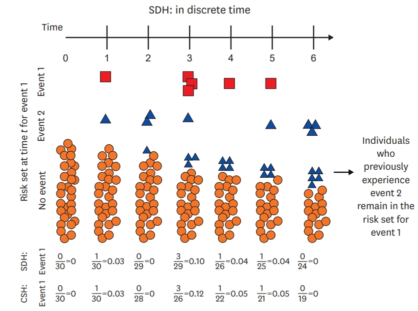
- There are two methods that can be used to obtain hazard ratio (HR) considering competing risks.5) First, the cause-specific hazard (CSH) function calculates HR for patients who are at risk of the event of interest (Figure 1). This method treats other outcomes as censored except the event of interest and uses the Cox regression based on a specific event. Thus, the CSH model is most commonly used for etiological research. The second method is the subdistribution hazard (SDH) function suggested by Fine and Gray (Figure 2).6)7) In this method, subjects who have experienced competing events are not censored but remain in risk sets. In other words, this includes subjects who have experienced competing events even if they are not at risk of the event of interest. The Fine and Gray model is appropriate for prognostic study or predicting an individual's risk.
HAZARD REGRESSION FUNCTION
- In the absence of competing risks, the traditional hazard function is defined as below.
- where S(t)=∫0th(s)ds, which is survival function.
- The hazard function describes the instantaneous rate of occurrence of the event of interest in subjects who are still at risk of the event. The Cox proportional hazard regression model can express the hazard function with covariates.
- where Χ and β are vectors of covariates and coefficients, respectively. If all covariates are equal to zero, covariates have no effect on the hazard function. In that case, the survival function is h0(t) which is a baseline hazard function. The HR from this function is eβ and can be interpreted as a relative change of risk with a 1-unit increase of an explanatory variable. The hazard function can be expressed by the survival function. S(t)=S0(t)exp(χβ), S0(t) being the baseline survival function. Estimating the effect of covariates on the risk of outcomes is equal to that on the log survival function. Therefore, estimation by the survival function and the estimation by the risk function have the same context.
- On the other hand, when several types of outcomes exist or the event of interest is censored by other outcomes, the estimation of the incidence of the primary outcome is disrupted. Standard survival analysis in which competing events are right-censored should not be applied. In the presence of competing risks, there are two suggestions of hazard regression: the CSH model and the SDH model.
- CSH model
- The CSH function denotes the instantaneous rate of the incidence of the kth event in subjects who are currently event-free. The risk set of the CSH function consists of subjects who have not yet experienced any type of events until time point t. If cardiovascular death and non-cardiovascular death are both considered, the CSH for cardiovascular death is the rate of cardiovascular death in subjects who have never experienced either event (i.e., subjects who are still alive).
- SDH model
- The model above shows the SDH function suggested by Fine and Gray (1999). This method uses the hazard of the subdistribution, which is a function of the cumulative incidence in each event. This function denotes the instantaneous rate of incidence of the kth event in subjects who have not experienced the kth event. In this model, not only subjects who are event-free, but also subjects who have experienced competing events before time t are kept in the risk set. This is different from the CSH function. Consistent with the example above, the SDH for cardiovascular death is the rate of cardiovascular death in subjects who are still alive or who are dead due to a non-cardiovascular cause.8-11) One needs to be mindful of the interpretation of the hazard ratio due to the risk set.
- In the presence of competing risks, these two different hazard functions can yield distinct hazard functions for each event. Although both models take competing risks into account, different hazard functions are used, resulting in the different interpretations of the effect of covariates. Lau et al.12) suggested that the CSH model is suitable for etiologic research, whereas the SDH model is for predicting an individual's risk. Valid estimates of regression coefficients can be obtained without assuming independence between competing events and the event of interest, since the CSH model censors all but the event of interest. This model also has the advantage of being easy to fit within any type of statistical software. However, it should be noted that patients at risk are reduced in follow-up studies. The CSH can be interpreted as the incidence rate of the event of interest in subjects who have not yet experienced any type of events. On the other hand, subjects who experienced competing events are still in risk sets in the SDH model. Consequently, the SHR from the subdistribution method cannot be interpreted as traditional HR. For example, when calculating HR for cardiovascular death, subjects who have died of non-cardiovascular causes are included in the risk set. This is contradictory because people only die once. However, the cumulative incidence of events can be predicted through a relationship between hazard and incidence function. In addition, even if predicting incidence is not the main purpose, this model allows one to estimate the effect of covariates on the CIF for the event of interest.
EXAMPLE USING SAS
- Bone marrow transplantation (BMT) is a standard treatment for acute leukemia. In 1997, the BMT dataset presented by Klein and Moeschberger,13) which is one of the most famous examples of competing risk analysis. This dataset contains data from 137 patients who went through transplantation. During the follow-up period, patients might relapse or die, or experience neither event. The variable Disease indicates the status of patients at the time of transplantation; acute lymphoblastic leukemia (ALL), acute myelocytic leukemia (AML) low-risk, and AML high-risk.
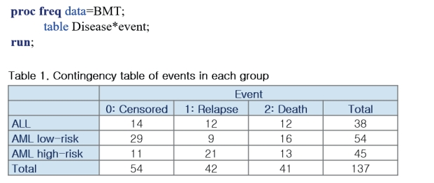
- The variable Dftime is the time from transplantation to the occurrence of either relapse or death. The variable event is coded as 0 for censored, 1 for relapse, and 2 for death before relapse. In this data, relapse is the event of interest and death is the competing event. The table shows the frequency of events in each group (Figure 3).
- First, check the rate of incidence of relapse without considering the competing event (Figure 4). PROC PHREG estimates the HR for each group of patients and shows that the HR of the AML low-risk group compared to ALL is 0.563 (p=0.0457) and that of the AML high-risk group compared to ALL is 1.466 (p=0.1524).
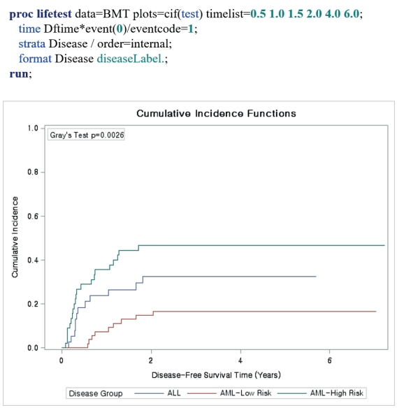
- Now, consider death as a competing event (Figure 5). The CIF can be estimated using PROC LIFETEST. Specify plots=cif and option eventcode=1 in the time statement. To estimate the CIF of death, designate eventcode as 2. The difference in the incidence of relapse among three groups is significant (p=0.0026).
- The HR of the SDH function can be estimated in PROC PHREG (Figure 6) with the same option above, eventcode=1 (which is the code of the event of interest, i.e., relapse). The SHR for the AML low-risk group is 0.448 (p=0.0608) and that for the AML high-risk group is 1.663 (p=0.1649).
- The CSH model can be fitted by specifying the event that would be censored (Figure 7). The code to be censored is defined in the model statement as Dftime*event(0,2)=Disease. The CSH for the AML low-risk group was 0.409 (p=0.0432) and that of the AML high-group was 1.840 (p=0.0921). As a result, HR for the AML low-risk group (0.563) in the general Cox regression was higher than SHR (0.448) and CSH (0.409). This implies that the general survival analysis overestimates the incidence of relapse by ignoring competing risks (in this case, death).
- R provides several packages to conduct competing risk analysis. The CIF can be estimated in R using the ‘cumincí’ function in the ‘cmprsk’ package. The ‘coxph’ function in the ‘survival’ package can be used for CSH regression and the ‘crr’ function in the ‘cmprsk’ package can be used for the SDH regression.
- STATA also allows CIFs to be estimated with the ‘stcurv’ function. The CSH model can be fit witht he ‘stcox’ function, and the SDH model with the ‘stcrreg’ function.
CONCLUSION
- When performing survival analysis, it is important to consider whether competing risks exist. The KM method and the Cox proportional hazard regression are the most widely used methods for analyzing survival probability during a study period. However, in the presence of competing risks, standard survival analysis methods may yield unreliable results in estimating survival probability. The use of CIF is recommended to calculate the incidence rate. Alternatives to the Cox proportional hazard regression are the CSH regression and the SDH regression. The former is suitable for etiological studies, while the latter is suitable for the prediction of an individual's survival probability.
ARTICLE INFORMATION
-
Conflict of Interest
The author has no financial conflicts of interest.
-
Author Contributions
Conceptualization: Lee WK; Formal analysis: Jeon Y; Methodology: Jeon Y, Lee WK; Supervision: Lee WK; Writing - original draft: Jeon Y; Writing - review & editing: Jeon Y, Lee WK.
Figure 1.
Overview of the calculation of the CSH. The risk set starts with 30 individuals (solid circles). Over time, individuals either experience event 1 (squares) or event 2 (triangles). As individuals experience either event, they are removed from the remaining risk sets. The calculation for the cause-specific hazard is given at the bottom of the figure from Lau et al.9)
CSH = cause-specific hazard.

Figure 2.
Overview of the calculation of the SDH. The risk set starts with 30 individuals (solid circles). Over time, individuals either experience event 1 (squares) or event 2 (triangles). When individuals experience a competing event (event 2, triangles), they are maintained in the risk set as triangles. Thus, over time, a greater proportion of the risk set becomes full of triangles, which represent individuals who have experienced the competing event prior to that time. The SDH for event 1 is given near the bottom of the figure along with the CSH for event 1 for comparison. Note that because individuals are maintained in the risk set, the SDH tends to be lower than the CSH from Lau et al.9)
CSH = cause-specific hazard; SDH = subdistribution hazard.

Figure 3.
SAS example (1).
ALL = acute lymphoblastic leukemia; AML = acute myelocytic leukemia; BMT = bone marrow transplantation.

Figure 4.
SAS example (2).
AML = acute myelocytic leukemia; BMT = bone marrow transplantation.

Figure 5.
SAS example (3).
ALL = acute lymphoblastic leukemia; AML = acute myelocytic leukemia; BMT = bone marrow transplantation.

Figure 6.
SAS example (4).
AML = acute myelocytic leukemia; BMT = bone marrow transplantation.

Figure 7.
SAS example (5).
AML = acute myelocytic leukemia; BMT = bone marrow transplantation.

REFERENCES
- 1. Abdel-Qadir H, Fang J, Lee DS, Tu JV, Amir E, Austin PC, Anderson GM. Importance of considering competing risks in time-to-event analyses: application to stroke risk in a retrospective cohort study of elderly patients with atrial fibrillation. Circ Cardiovasc Qual Outcomes 2018;11:e004580.PubMedPMC
- 2. Glynn RJ, Rosner B. Comparison of risk factors for the competing risks of coronary heart disease, stroke, and venous thromboembolism. Am J Epidemiol 2005;162:975–82.ArticlePubMed
- 3. Feakins BG, McFadden EC, Farmer AJ, Stevens RJ. Standard and competing risk analysis of the effect of albuminuria on cardiovascular and cancer mortality in patients with type 2 diabetes mellitus. Diagn Progn Res 2018;2:13. ArticlePubMedPMC
- 4. Wolbers M, Koller MT, Witteman JC, Steyerberg EW. Prognostic models with competing risks: methods and application to coronary risk prediction. Epidemiology 2009;20:555–61.PubMed
- 5. Austin PC, Lee DS, Fine JP. Introduction to the analysis of survival data in the presence of competing risks. Circulation 2016;133:601–9.ArticlePubMedPMC
- 6. Fine JP, Gray RJ. A proportional hazards model for the subdistribution of a competing risk. J Am Stat Assoc 1999;94:496–509.Article
- 7. Austin PC, Fine JP. Practical recommendations for reporting Fine-Gray model analyses for competing risk data. Stat Med 2017;36:4391–400.ArticlePubMedPMC
- 8. Fanaroff AC, Roe MT, Clare RM, Lokhnygina Y, Navar AM, Giugliano RP, Wiviott SD, Tershakovec AM, Braunwald E, Blazing MA. Competing risks of cardiovascular versus noncardiovascular death during long-term follow-up after acute coronary syndromes. J Am Heart Assoc 2017;6:e005840.ArticlePubMedPMC
- 9. Huebner M, Wolkewitz M, Enriquez-Sarano M, Schumacher M. Competing risks need to be considered in survival analysis models for cardiovascular outcomes. J Thorac Cardiovasc Surg 2017;153:1427–31.ArticlePubMed
- 10. Warnock DG. Competing risks: you only die once. Nephrol Dial Transplant 2016;31:1033–5.ArticlePubMedPMC
- 11. Noordzij M, Leffondré K, van Stralen KJ, Zoccali C, Dekker FW, Jager KJ. When do we need competing risks methods for survival analysis in nephrology? Nephrol Dial Transplant 2013;28:2670–7.ArticlePubMed
- 12. Lau B, Cole SR, Gange SJ. Competing risk regression models for epidemiologic data. Am J Epidemiol 2009;170:244–56.ArticlePubMedPMC
- 13. Klein JP, Moeschberger ML. Survival Analysis: Techniques for Censored and Truncated Data. New York, NY, Springer; 1997.
Citations
Citations to this article as recorded by

- People with genetic kidney diseases on kidney replacement therapy have different clinical outcomes compared to people with other kidney diseases
Helen Y. Han, Venkat Vangaveti, Matthew Jose, Monica Suet Ying Ng, Andrew John Mallett
Scientific Reports.2024;[Epub] CrossRef - Factor modification in the association between high-density lipoprotein cholesterol and liver cancer risk in a nationwide cohort
Su Youn Nam, Junwoo Jo, Won Kee Lee, Chang Min Cho
International Journal of Epidemiology.2024;[Epub] CrossRef - Standard Survival Analysis Can Overestimate Incidence and Risk Factors of Event of Interest in a Prospective Cohort Study with Considerable Attrition: The Case of a Suicide High-Risk Cohort
Min Ji Kim, Maengseok Noh, Jieun Yoo, Seung Yeon Jeon, Jungjoon Moon, Seong Jin Cho, Sang Yeol Lee, Se-Hoon Shim, Shin Gyeom Kim, Won Sub Kang, Min-Hyuk Kim, Christopher Hyung Keun Park, Daun Shin, Sang Jin Rhee, Jeong Hun Yang, Yong-Min Ahn, Weon-Young L
SSRN Electronic Journal .2022;[Epub] CrossRef
 , Won Kee Lee, PhD

